An Illustrated Tour of Wav2vec 2.0
Transformer-based neural networks have been revolutionizing the natural language processing field, but are only starting to become popular in the speech processing community. Wav2vec 2.0 is set to change that. Its architecture is based on the Transformer’s encoder, with a training objective similar to BERT’s masked language modeling objective, but adapted for speech.
This new method allows for efficient semi-supervised training: first, pre-train the model on a large quantity of unlabeled speech, then fine-tune on a smaller labeled dataset. In wav2vec 2.0’s original paper, the authors demonstrated that fine-tuning the model on only one hour of labeled speech data could beat the previous state-of-the-art systems trained on 100 times more labeled data.
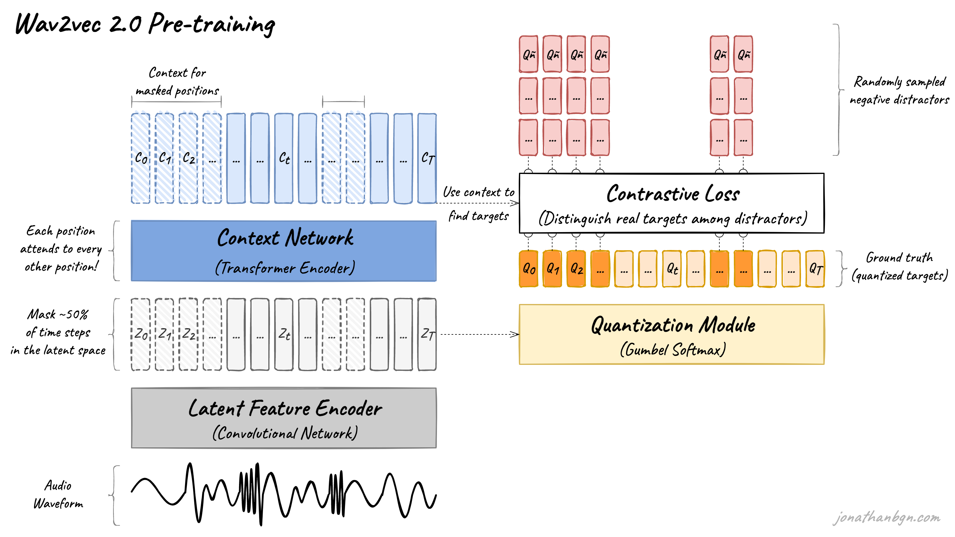
Above is an overview of the wav2vec 2.0 architecture and its pre-training process. There are four important elements in this diagram: the feature encoder, context network, quantization module, and the contrastive loss (pre-training objective). We will open the hood and look in detail at each one.
Feature encoder
The feature encoder’s job is to reduce the dimensionality of the audio data, converting the raw waveform into a sequence of feature vectors Z0, Z1, Z2, …, ZT each 20 milliseconds. Its architecture is simple: a 7-layer convolutional neural network (single-dimensional) with 512 channels at each layer.
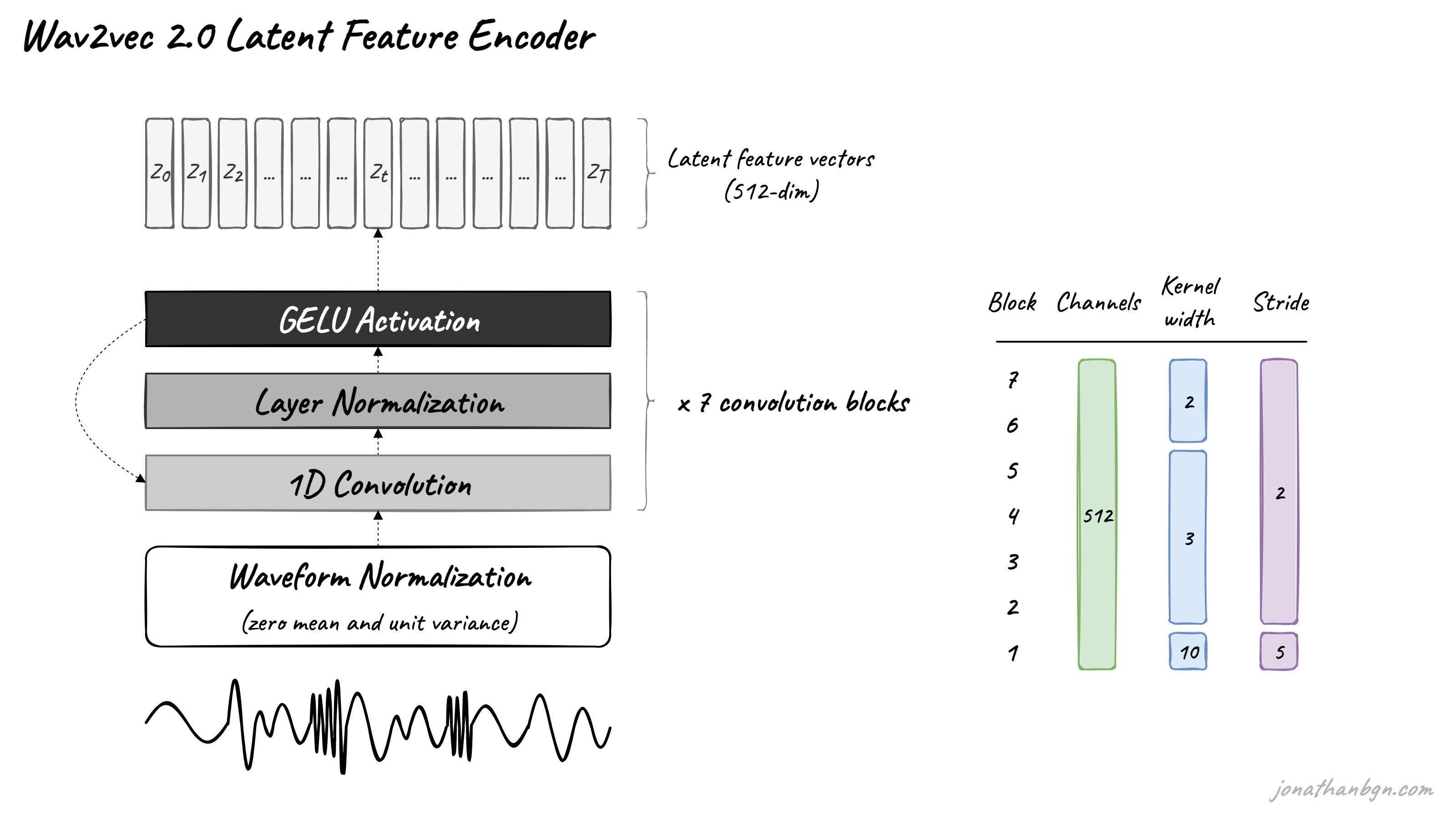
The waveform is normalized before being sent to the network, and the kernel width and strides of the convolutional layers decrease as we get higher in the network. The feature encoder has a total receptive field of 400 samples or 25 ms of audio (audio data is encoded at a sample rate of 16 kHz).
Quantization module
One of the main obstacles of using Transformers for speech processing is the continuous nature of speech. Written language can be naturally discretized into words or sub-words, therefore creating a finite vocabulary of discrete units. Speech doesn’t have such natural sub-units. We could use phones as a discrete system, but then we would need humans to first label the entire dataset beforehand, so we wouldn’t be able to pre-train on unlabeled data.
Wav2vec 2.0 proposes to automatically learn discrete speech units, by sampling from the Gumbel-Softmax distribution. Possible units are made of codewords sampled from codebooks (groups). Codewords are then concatenated to form the final speech unit. Wav2vec uses 2 groups with 320 possible words in each group, hence a theoretical maximum of 320 x 320 = 102,400 speech units.
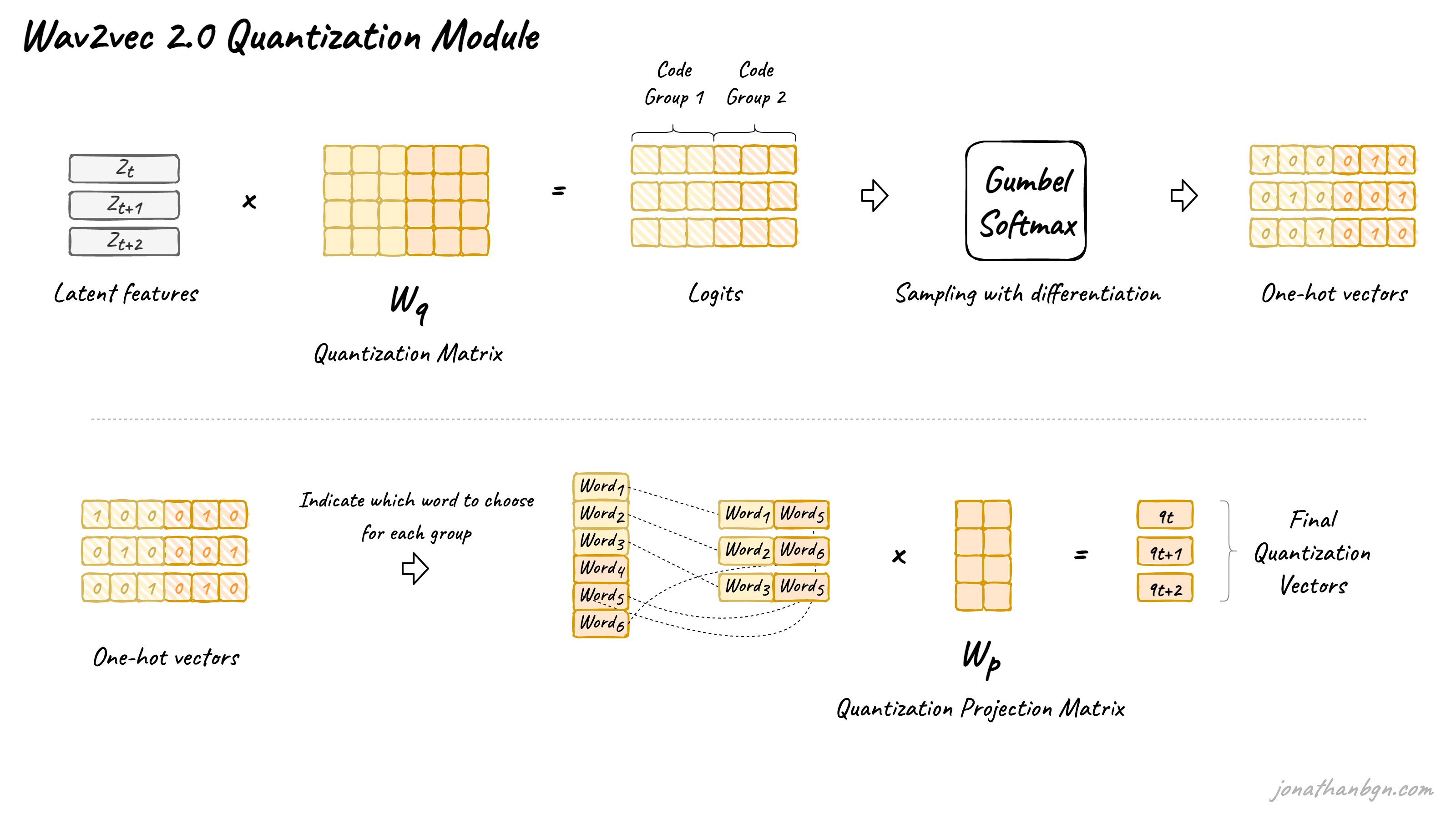
The latent features are multiplied by the quantization matrix to give the logits: one score for each of the possible codewords in each codebook. The Gumbel-Softmax trick allows sampling a single codeword from each codebook, after converting these logits into probabilities. It is similar to taking the argmax except that the operation is fully differentiable. Moreover, a small randomness effect, whose effect is controlled by a temperature argument, is introduced to the sampling process to facilitate training and codewords utilization.
Context network
The core of wav2vec 2.0 is its Transformer encoder, which takes as input the latent feature vectors and processes it through 12 Transformer blocks for the BASE version of the model, or 24 blocks for the LARGE version. To match the inner dimension of the Transformer encoder, the input sequence first needs to go through a feature projection layer to increase the dimension from 512 (output of the CNN) to 768 for BASE or 1,024 for LARGE. I will not describe further the Transformer architecture here and invite you to read The Illustrated Transformer if you forgot the details.
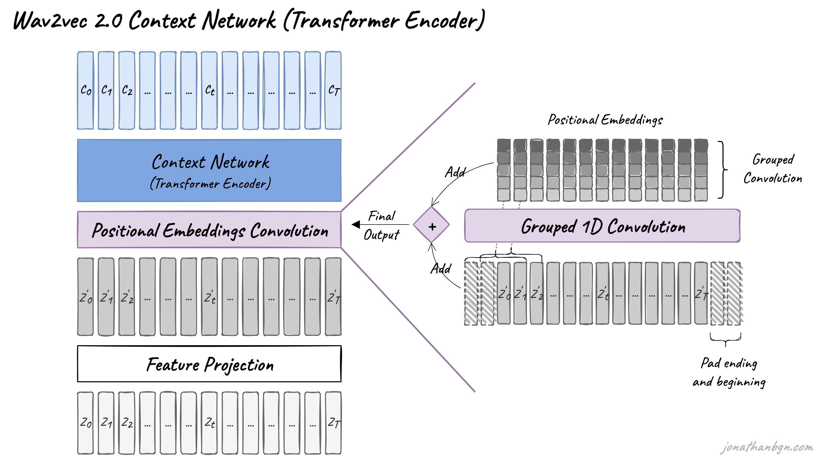
One difference from the original Transformer architecture is how positional information is added to the input. Since the self-attention operation of the Transformer doesn’t preserve the order of the input sequence, fixed pre-generated positional embeddings were added to the input vectors in the original implementation. The wav2vec model instead uses a new grouped convolution layer to learn relative positional embeddings by itself.
Pre-training & contrastive loss
The pre-training process uses a contrastive task to train on unlabeled speech data. A mask is first randomly applied in the latent space, where ~50% of the projected latent feature vectors. Masked positions are then replaced by the same trained vector Z’M before being fed to the Transformer network.
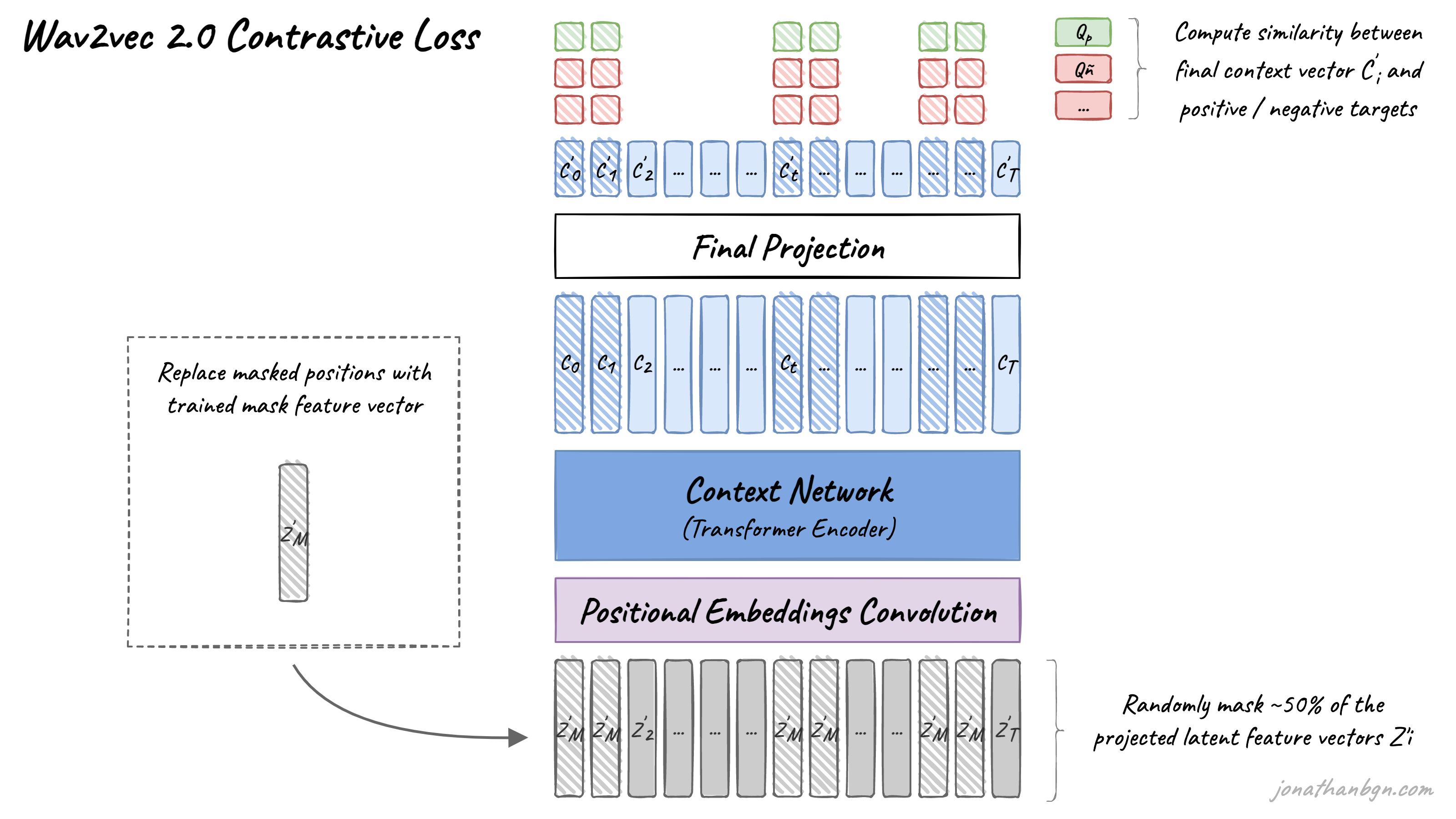
The final context vectors then go through the last projection layer to match the dimension of the quantized speech units Qt. For each masked position, 100 negative distractors are uniformly sampled from other positions in the same sentence. The model then compares the similarity (cosine similarity) between the projected context vector C’t and the true positive target Qp along with all negative distractors Qñ. The contrastive loss then encourages high similarity with the true positive target and penalizes high similarity scores with negative distractors.
Diversity loss
During pre-training, another loss is added to the contrastive loss to encourage the model to use all codewords equally often. This works by maximizing the entropy of the Gumbel-Softmax distribution, preventing the model to always choose from a small sub-group of all available codebook entries. You can find more details in the original paper.
Conclusion
This concludes our tour of wav2vec 2.0 and its pre-training process. The resulting pre-trained model can be used for a variety of speech downstream tasks: automatic speech recognition, emotion detection, speaker recognition, language detection… In the original paper, the authors directly fine-tuned the model for speech recognition with a CTC loss, adding a linear projection on top of the context network to predict a word token at each timestep.
Read next
HuBERT: How to Apply BERT to Speech, Visually Explained