The Illustrated Wav2vec
Wav2vec is a speech encoder model released by the Facebook AI team in late 2019. It quickly became popular in the speech processing community as it enabled new state-of-the-art performance for various speech tasks like automatic speech recognition or emotion recognition. Since its original version, the model has been upgraded to use the Transformers architecture (the same one behind GPT and BERT) and has been re-trained on 12 different languages in a multilingual version.
I haven’t seen resources digging into the internals of the model, so I decided to write this short illustrated tour, inspired by the excellent Illustrated GPT article.
Like GPT, but for speech
Wav2vec is a big deal because it is one of the most promising attempts so far to apply self-supervised learning to the field of speech processing. It has the potential to change best practices in the field, just like GPT and BERT changed the field of natural language processing.
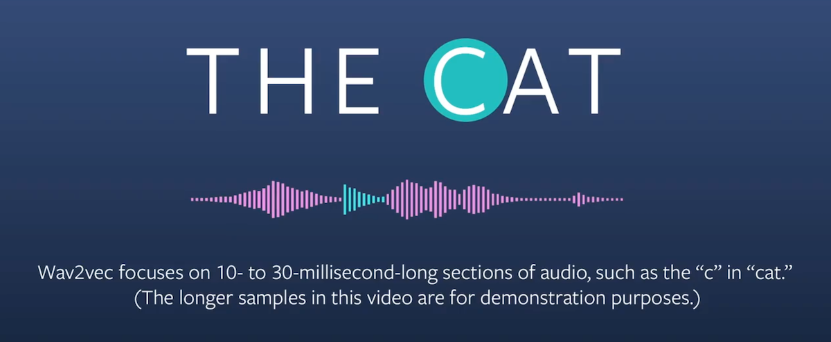
Similar to GPT-2 or GPT-3 for text, wav2vec is trying to predict the future of an audio sequence, although through a different approach. Despite technical differences, the purpose of both models is identical. First, pre-train a large network on unlabeled data to learn useful contextual representations of the text/audio sequence. Second, use these pre-trained representations for a variety of tasks for which not enough data is available.
 Source: Facebook AI Blog
There are however challenges to model the future of audio sequences compared to text. Audio data has a much higher dimension than text (text has a finite vocabulary), so directly modeling the waveform signal is much harder. Instead, wav2vec first reduces the dimensionality of the speech data by encoding it into a latent space, and then predicting the future in this latent space.
Let’s open the hood and look at the model architecture to see how this is done.
Dual model architecture: encoder & context network
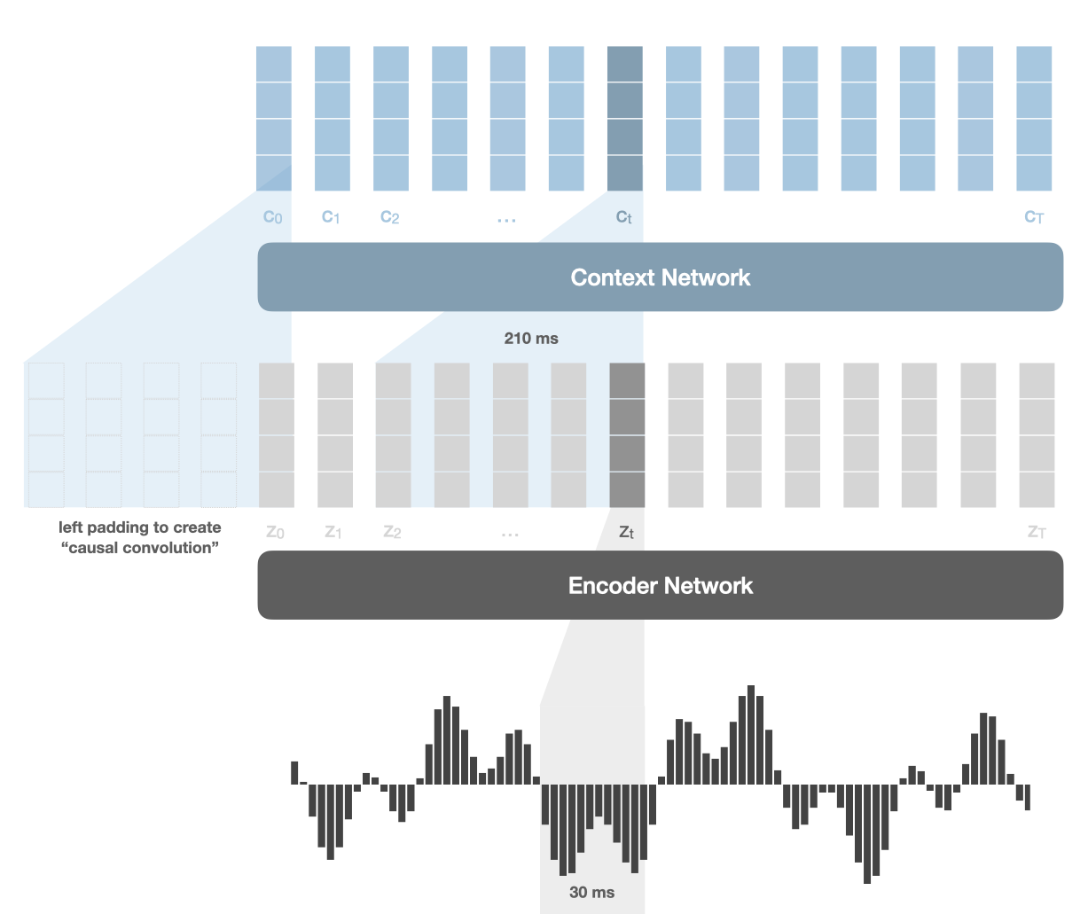
At the core of wav2vec are two distinct networks: the encoder network and the context network. Both are convolutional neural networks, albeit with different settings.
The encoder network reduces the dimensionality of the speech data, by encoding 30 milliseconds of audio into a 512-dimensional feature vector zt at each timestep t, every 10 ms.
The context network takes as input the encoder output features, encoding 210 ms of raw audio into another 512-dimensional feature vector ct. The objective is to aggregate information over a longer timeframe to model higher-order information. This network outputs contextual representations ct that are used to predict future audio samples.
An important detail is the causal nature of these convolutional networks. Wav2vec should not “peek” into the future when predicting future samples, hence the convolutional layers are structured in a way that each output at time t never attends to positions after t. In practice, this is done through left-padding the input as shown in the diagram below.
Maximizing mutual information
The idea behind wav2vec training is called contrastive predictive coding. Instead of trying to predict directly the future like GPT and model precisely the audio waveform, wav2vec uses a contrastive loss that implicitly models the mutual information between the context and future audio samples.
Mutual information is a concept coming from information theory which indicates how much information is gained about a given random variable when we observe another random variable. If the mutual information is 0, the two variables are independent. If it is 1, then knowing about one variable will tell us everything we need to know about the other.

Wav2vec’s loss has been designed to implicitly maximize the mutual information between the context features and future audio samples. Doing so will push the model to learn useful contextual features which contain higher-order information about the audio signal.
If you want to know more about how wav2vec loss implicitly maximizes the mutual information, you can have a look at the contrastive predictive coding paper. This talk at NeurIPS by one of the authors also gives the intuition behind the concept.
Let’s now see how this loss objective is implemented in practice.
Training objective
The model is trained to distinguish true future audio samples from fake distractor samples by using the context vector. Here “audio samples” actually mean the encoder feature vectors zi. Remember that we are not working with the waveform directly because the dimensionality would be too high. This prediction process is done k times at each timestep t, for each one of k=12 steps in the future.
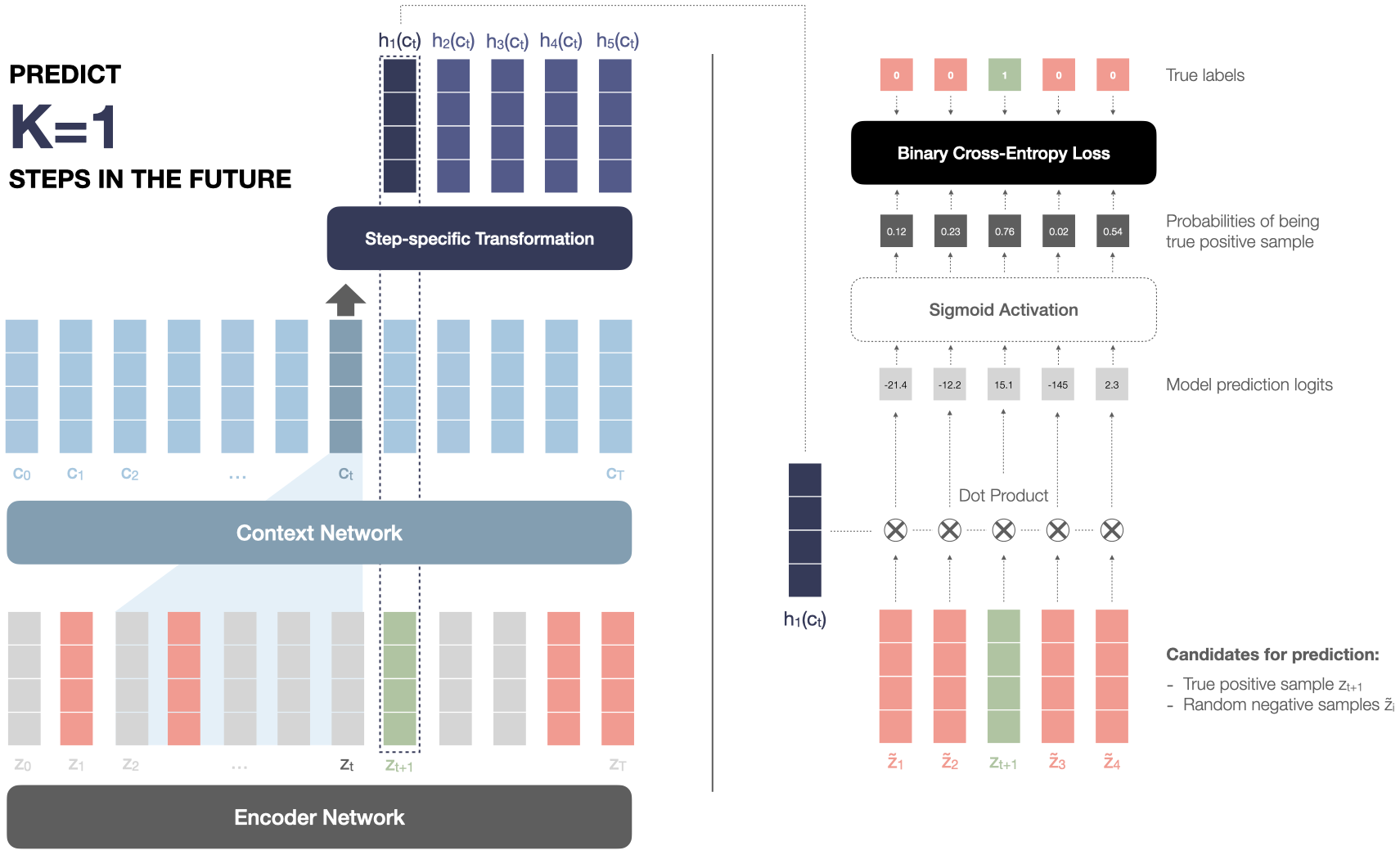
Concretely, at a given timestep t, for each step k = 1 … 12, we do the following:
- Extract the true audio sample zt+k at future step k
- Pick 10 random negative samples z̃1..10 from the same audio sequence
- Compute a step k-specific transformation hk(ct) of the context vector at time t
- Compute the similarity (dot product) of the transformed context vector with all z candidates
- Compute the final probabilities of positive/negative through a sigmoid activation
- Compare with the ground truth and penalize the model for wrong predictions (binary cross-entropy loss)
The following illustrates this process for the step k=1 (only four negatives are represented for simplicity):
And here is the same thing but for step k=2 for a better understanding of the process:
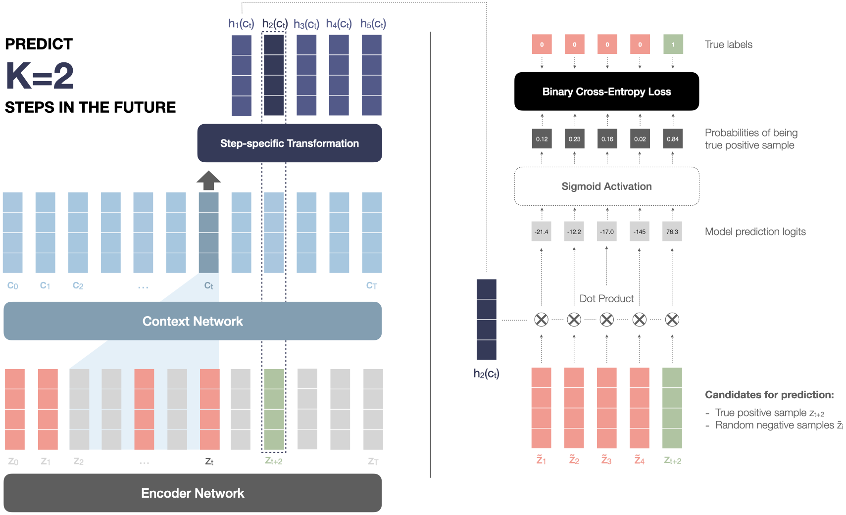
The output of the model is the model computed probabilities for each sample to be the true future sample. A final binary cross-entropy loss is applied to penalize the model for wrongly predicting a negative sample as positive and vice versa. The total loss is the sum of the individual losses at each timestep t for each future step k in the future:

Future applications
In the original paper, the authors used wav2vec pre-trained representations as input for a separate speech recognition model. They demonstrated the power of their method by improving the previous best accuracy by 22% while using two orders of magnitude less labeled data.
However, the use of wav2vec embeddings isn’t limited to speech recognition only. In a previous blog post, I wrote about how using wav2vec embeddings allowed us to improve speech emotion recognition accuracy while using less labeled data for training. There is also potential to apply to more tasks like speech translation, speaker recognition, speaker diarization, etc.
Read next
Detecting Emotions from Voice with Very Few Training Data